Kerasではじめての二値分類
今日はKerasでロジスティック回帰をし、二値分類してみる。
○と×にラベル付けされたデータがあるときに、 ○と×をうまく分ける条件(決定境界)を求めるのが二値分類の課題。
この問題でよく紹介されるのは二次元空間上のデータを直線で分離するケースだが、 本稿ではちょっとがんばって決定境界が円になるケースを解いてみる。
事前準備
とりあえずKerasライブラリをインポートする。
import matplotlib
matplotlib.use("Agg")
import matplotlib.pyplot as plt

from keras.models import Sequential
from keras.layers import Dense, Activation
from keras.callbacks import EarlyStopping

import numpy as np
次に、学習させるデータを用意する。 今回も数学的につくってしまうことにする。
本日のお題にする決定境界関数は、以下。
\[\frac{(X_0 - p)^2}{a^2} + \frac{(X_1 - q)^2}{b^2} > 1\]楕円だね。楕円の内側を当り(○)、外側を外れ(×)ということにする。
各パラメータは次のPythonプログラムの通り:
def f(x_0, x_1):
  p = 0.6
  q = 0.4
  a2 = 0.3 ** 2
  b2 = 0.3 ** 2
  return ((x_0 - p) ** 2) / a2 + ((x_1 - q) ** 2) / b2 > 1
実際に○×データを生成する。
X = np.random.random((10000, 2))
y = f(X[:,0], X[:,1]) + 0

X_train = X[:9000]
y_train = y[:9000]
X_test = X[9001:]
y_test = y[9001:]
可視化する。
plt.clf()
X_positive = X_train[np.where(y_train == 0)]
X_negative = X_train[np.where(y_train == 1)]
plt.plot(X_positive[:500,0], X_positive[:500,1], 'o')
plt.plot(X_negative[:500,0], X_negative[:500,1], 'x')
plt.savefig('X_train.png')
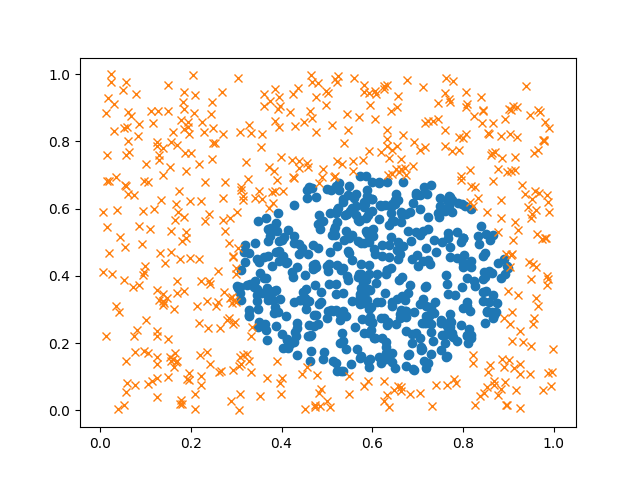
ちょっときもい。
モデル構築
先ほどの○×分布を見ると、明らかに二次関数である。 そこで、\(X\) を拡張して、二乗の値も入力値に入れておく。
X = np.c_[A[:,0], A[:,1], A[:,0]**2, A[:,1]**2]
こうしておくことで、学習により推定するパラメータ \(\theta\) と \(X\) は 以下のような関係になる。
\[\begin{align} \theta^T X + b &= 0 \\ \begin{bmatrix} \theta_0 & \theta_1 & \theta_2 & \theta_3 \end{bmatrix} \begin{bmatrix} X_0 \\ X_1 \\ X_0^2 \\ X_1^2 \end{bmatrix} + b &= 0 \end{align}\]ロジスティック回帰を使った二値分類では 目的関数 \(J(\theta)\) を以下のように定義して、 \(J(\theta)\) が最小になる \(\theta\) を学習により求める。
\[J(\theta) = - \frac{1}{m} \sum_{i=0}^{m-1} y \log(h_\theta(X)) + (1-y) \log(1 - h_\theta(X))\]真ん中の式の説明は省略。
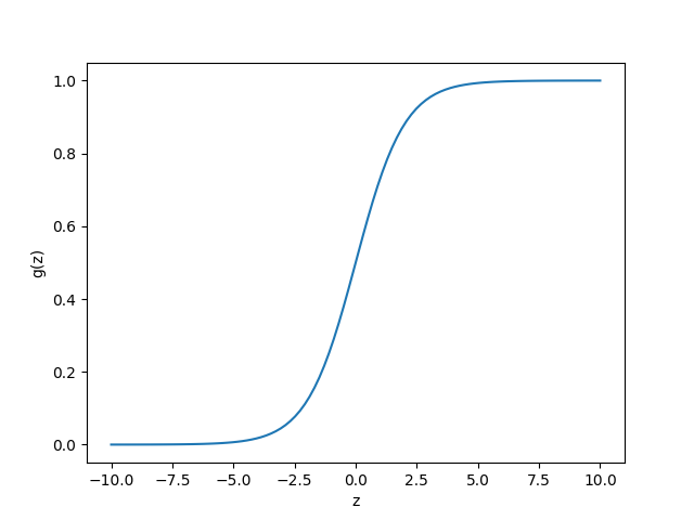
\(h_\theta(X)\) はシグモイド関数
\[g(z) = \frac{1}{1+e^{-z}}\]を使い、
\[h_\theta(X) = g(\theta^T x) = \frac{1}{1+e^{- \theta^T x}}\]とおく。 \(h_\theta(X)\) は 入力 \(X\) に対し、\(y = 1\) になる確率とみなせる。 すなわち、以下の式のように書く。
\[y = \begin{cases} \begin{array}{ll} 1 & (h_\theta(X) \geq 0.5) \\ 0 & (h_\theta(X) \lt 0.5) \end{array} \end{cases}\]ちなみにシグモイド関数は以下のような形になる。
plt.clf()
z = np.linspace(-10, 10, 102)
gz = 1 / (1 + np.exp(-z))
plt.xlabel('z')
plt.ylabel('g(z)')
plt.plot(z, gz)
plt.savefig('logistic.png')
なおKerasでロジスティック回帰するために、ここまでの式への理解は必須ではない。 ただ下記のようにプログラムを書くだけである。
model = Sequential()
model.add(Dense(1, input_dim=4, kernel_initializer='uniform'))
model.add(Activation('sigmoid'))
model.compile(optimizer='adam', loss='binary_crossentropy',
              metrics=['accuracy'])
学習開始
以下のようにプログラムを書き実行する。
early_stopping = EarlyStopping(monitor='val_loss', patience=2)
hist = model.fit(X_train, y_train,
                 epochs=1000, verbose=1,
                 validation_split=0.1,
                 callbacks=[early_stopping])
EarlyStopping(monitor='val_loss', patience=2) を
callbacks パラメータとして渡すと、val_lossが変化しなくなった時点で
学習を自動的に終了してくれる。
val_lossはバリデーションセットで評価した場合のコストを指す。
val_lossを終了判定の基準とするには、バリデーションセットの評価を有効にする必要がある。validation_split=0.1を引数に指定すると、訓練データセットのうち1割を自動でバリデーションセットとしてくれるらしい。
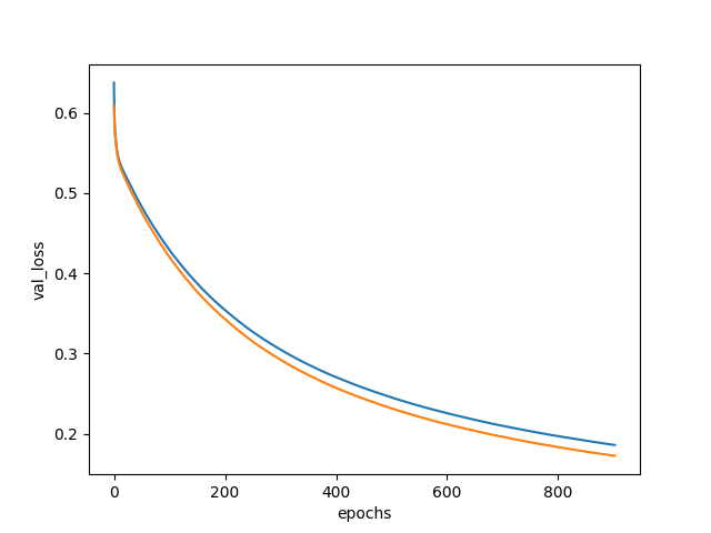
実行してみたところなかなか学習が進まなかったが、900周目で止まった。
学習曲線を描いてみた。
plt.clf()
plt.xlabel('epochs')
plt.ylabel('val_loss')
plt.plot(np.arange(0, 903), hist.history['loss'], label='loss')
plt.plot(np.arange(0, 903), hist.history['val_loss'], label='val_loss')
plt.savefig('fit_loss.png')
以下のようになった。
評価1
学習したパラメータについて、テストデータで評価してみる。
>>> scores = model.evaluate(X_test, y_test)
>>> print(scores)
[0.17704800366460383, 0.97497497497497498]
まあまあっぽい。
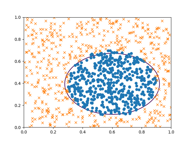
評価2: 決定境界線
決定境界を描いてみる。 描くだけならば、楕円のパラメータを求める必要は無い。
w = model.get_weights()
theta = w[0][:,0]
theta_0, theta_1, theta_2, theta_3 = theta
bias = w[1][0]

X_0_mesh = np.linspace(0, 1, 51)
X_1_mesh = np.linspace(0, 1, 51)
X_0_mesh, X_1_mesh = np.meshgrid(X_0_mesh, X_1_mesh)
y = X_0_mesh * theta_0 + X_1_mesh * theta_1 + (X_0_mesh ** 2) * theta_2 + (X_1_mesh ** 2) * theta_3 + bias

plt.clf()
X_positive = X_train[np.where(y_train == 0)]
X_negative = X_train[np.where(y_train == 1)]

plt.contour(X_0_mesh, X_1_mesh, y, [0])
plt.plot(X_positive[:500,0], X_positive[:500,1], 'o')
plt.plot(X_negative[:500,0], X_negative[:500,1], 'x')
plt.savefig('Xy_pred.png')
だいたいうまく分離できたようだ。
評価3: 精度、再現性
分類問題は単なる正答率だけでなく、 Precision、Recallという指標で評価するとよい、と先生が話していたのでやってみる。
Precisionは、正答が○であることを予測できた確率、 Recallは、正解したうち正答が○のものを拾えた確率、を表わしている。
この二つを合わせてF値というらしい。
これらは、正答と予測した答えについて True Positive、False Positive、False Negative、True Positiveの個数を数えれば計算できる。
| 正答 | 予測 | |
|---|---|---|
| True Positive | ○ | ○ |
| False Positive | ○ | × |
| False Negative | × | ○ |
| True Negative | × | × |
Precision、Recallは以下の式で計算する。
\[\begin{align} Precision &= \frac{\#TP}{\#TP + \#FP} \\ Recall &= \frac{\#TP}{\#TP + \#FN} \end{align}\]この計算プログラムは自作した。
class ThreatScore(object):
  def __init__(self, score=None):
    if score is not None:
      self.true_positive = score.true_positive
      self.false_positive = score.falsee_positive
      self.false_negative = score.false_negative
      self.true_negative = score.true_negative

  def calc(self, correct, pred):
    self.true_positive = np.sum(np.logical_and(correct == 1, pred == 1))
    self.false_positive = np.sum(np.logical_and(correct == 0, pred == 1))
    self.false_negative = np.sum(np.logical_and(correct == 1, pred == 0))
    self.true_negative = np.sum(np.logical_and(correct == 0, pred == 0))

  def __str__(self):
    t = 'TP: {}, FP: {}, FN: {}, TN: {}'
    return t.format(self.true_positive, self.false_positive, self.false_negative, self.true_negative)

def precision(v):
  return v.true_positive * 1.0 / (v.true_positive + v.false_positive)

def recall(v):
  return v.true_positive * 1.0 / (v.true_positive + v.false_negative)
それではPrecision、Recallを計算してみる。
v = ThreatScore()
y_pred = (X_test[:,0] * theta_0 + X_test[:,1] * theta_1 + (X_test[:,0] ** 2) * theta_2 + (X_test[:,1] ** 2) * theta_3 + bias > 0) + 0
y_pred = y_pred + 0
v.calc(y_test, y_pred)
結果は以下の通り。 かなり予測できたっぽい。めでたしめでたし。
print('Precision: {}, Recall: {}'.format(precision(v), recall(v)))
Precision: 0.972451790634, Recall: 0.986033519553
ソースコード
最後にソースコードを貼り付けておく。
import matplotlib
matplotlib.use("Agg")
import matplotlib.pyplot as plt

from keras.models import Sequential
from keras.layers import Dense, Activation
from keras.callbacks import EarlyStopping

import numpy as np

def f(x_0, x_1):
  p = 0.6
  q = 0.4
  a2 = 0.3 ** 2
  b2 = 0.3 ** 2
  return ((x_0 - p) ** 2) / a2 + ((x_1 - q) ** 2) / b2 > 1.0

# Prepare data
A = np.random.random((10000, 2))
X = np.c_[A[:,0], A[:,1], A[:,0]**2, A[:,1]**2]
y = f(X[:,0], X[:,1]) + 0

A_train = A[:9000]
X_train = X[:9000]
y_train = y[:9000]
X_test = X[9001:]
y_test = y[9001:]

plt.clf()
X_positive = X_train[np.where(y_train == 0)]
X_negative = X_train[np.where(y_train == 1)]
plt.plot(X_positive[:500,0], X_positive[:500,1], 'o')
plt.plot(X_negative[:500,0], X_negative[:500,1], 'x')
plt.savefig('X_train.png')

# Build a model
model = Sequential()
model.add(Dense(1, input_dim=4, kernel_initializer='uniform'))
model.add(Activation('sigmoid'))
model.compile(optimizer='adam', loss='binary_crossentropy',
              metrics=['accuracy'])

# Run training
early_stopping = EarlyStopping(monitor='val_loss', patience=2)
hist = model.fit(X_train, y_train,
                 epochs=1000, verbose=1,
                 validation_split=0.1,
                 callbacks=[early_stopping])

plt.clf()
plt.xlabel('epochs')
plt.ylabel('val_loss')
plt.plot(np.arange(0, 903), hist.history['loss'], label='loss')
plt.plot(np.arange(0, 903), hist.history['val_loss'], label='val_loss')
plt.savefig('fit_loss.png')

scores = model.evaluate(X_test, y_test)
print(scores)

# Show result
w = model.get_weights()
theta = w[0][:,0]
theta_0, theta_1, theta_2, theta_3 = theta
bias = w[1][0]

print('theta_0 = {}, theta_1 = {}, theta_2 = {}, theta_3 = {}, bias = {}'
      .format(theta_0, theta_1, theta_2, theta_3, bias)

X_0_mesh = np.linspace(0, 1, 51)
X_1_mesh = np.linspace(0, 1, 51)
X_0_mesh, X_1_mesh = np.meshgrid(X_0_mesh, X_1_mesh)
y_mesh = X_0_mesh * theta_0 + X_1_mesh * theta_1 + (X_0_mesh ** 2) * theta_2 + (X_1_mesh ** 2) * theta_3 + bias

plt.clf()
X_positive = X_train[np.where(y_train == 0)]
X_negative = X_train[np.where(y_train == 1)]
plt.contour(X_0_mesh, X_1_mesh, y_mesh, [0])
plt.plot(X_positive[:500,0], X_positive[:500,1], 'o')
plt.plot(X_negative[:500,0], X_negative[:500,1], 'x')
plt.savefig('Xy_pred.png')

class ThreatScore(object):
  def __init__(self, score=None):
    if score is not None:
      self.true_positive = score.true_positive
      self.false_positive = score.falsee_positive
      self.false_negative = score.false_negative
      self.true_negative = score.true_negative

  def calc(self, correct, pred):
    self.true_positive = np.sum(np.logical_and(correct == 1, pred == 1))
    self.false_positive = np.sum(np.logical_and(correct == 0, pred == 1))
    self.false_negative = np.sum(np.logical_and(correct == 1, pred == 0))
    self.true_negative = np.sum(np.logical_and(correct == 0, pred == 0))

  def __str__(self):
    t = 'TP: {}, FP: {}, FN: {}, TN: {}'
    return t.format(self.true_positive, self.false_positive, self.false_negative, self.true_negative)

def precision(v):
  return v.true_positive * 1.0 / (v.true_positive + v.false_positive)

def recall(v):
  return v.true_positive * 1.0 / (v.true_positive + v.false_negative)

v = ThreatScore()
y_pred = (X_test[:,0] * theta_0 + X_test[:,1] * theta_1 + (X_test[:,0] ** 2) * theta_2 + (X_test[:,1] ** 2) * theta_3 + bias > 0) + 0
y_pred = y_pred + 0
v.calc(y_test, y_pred)
print('Precision: {}, Recall: {}'.format(precision(v), recall(v)))